Using Keras to Identify an ARX model of a Dynamical System

In this post, we are going to show how to identify an autoregressive exogenous (ARX) model of a dynamical system. To perform the identification task we use a multilayer perceptron (MLP) network architecture implemented in Keras.

For impatient, the codes can be found here.

In our previous post, we have shown how to identify a model using recurrent neural networks and Keras. In that post, we have only used the dynamical system’s input to perform the identification and we have seen that a model of a relatively high order (for example Keras’s simpleRNN layer of the order 32) is necessary to estimate the model. Here we see that if use both observed outputs and inputs of the dynamical system, then we can relatively accurately estimate the ARX model using a low-dimensional MLP.

Often in the literature, the starting point for the development of the neural network identification procedure is an ARX model. However, to readers without strong control theory background, the connection between state-space and ARX models is unclear. To explain this connection, let us start from a discrete-time system:

$$\begin{align} & \mathbf{x}_{k+1}=A\mathbf{x}_{k}+B\mathbf{u}_{k} \label{eq1:stateDiscrete} \\ & \mathbf{y}_{k}=C\mathbf{x}_{k}+ D\mathbf{u}_{k}\label{eq1:outputDiscrete} \end{align}$$

where $k$ is the discrete time instant, $\mathbf{x}_{k}\in\mathbb{R}^{n}$, $\mathbf{y}_{k}\in\mathbb{R}^{r}$, $\mathbf{u}_{k} \in \mathbb{R}^{n}$, are the state, observed output, and external input vectors, and $A$, $B$, and $C$ are the system matrices. From \eqref{eq1:stateDiscrete} and \eqref{eq1:outputDiscrete} we have:

$$\begin{align} & \mathbf{y}_{k}=C\mathbf{x}_{k} \label{eq2:lifted1} \\ & \mathbf{y}_{k+1}=CA \mathbf{x}_{k} +CB \mathbf{u}_{k} \label{eq2:lifted2} \\ & \mathbf{y}_{k+2}=CA^2 \mathbf{x}_{k} +CAB \mathbf{u}_{k} +CB \mathbf{u}_{k+1} \label{eq2:lifted3} \end{align}$$

Proceeding in the same manner, we obtain the following equation:

$$\begin{align} \mathbf{y}_{k:k+p}=O_{p}\mathbf{x}_{k}+ M_{p}\mathbf{u}_{k:k+p} \label{liftedEquation} \end{align}$$

where

$$\begin{align} \mathbf{y}_{k:k+p}= \begin{bmatrix} \mathbf{y}_{k} \\ \mathbf{y}_{k+1} \\ \mathbf{y}_{k+2} \\ \vdots \\ \mathbf{y}_{k+p} \end{bmatrix}, \mathbf{u}_{k:k+p}= \begin{bmatrix} \mathbf{u}_{k} \\ \mathbf{u}_{k+1} \\ \mathbf{u}_{k+2} \\ \vdots \\ \mathbf{u}_{k+p} \end{bmatrix}, O_{p}=\begin{bmatrix}C \\ CA \\CA^2 \\ \vdots \\ CA^{p} \end{bmatrix}, M_{p}=\begin{bmatrix} 0 & 0 & 0 & \ldots & 0 \\ CB & 0 & 0 & \ldots & 0 \\ CAB & CB & 0 & \ldots & 0 \\ \vdots & \vdots & & & \vdots \\ CA^{p-1}B & CA^{p-2}B & \ldots & CB & 0\end{bmatrix} \label{liftedMatrices} \end{align}$$

The system representation \eqref{liftedEquation}-\eqref{liftedMatrices} is often referred to as the lifted system representation. The positive integer $p$ is referred to as the past horizon. The vectors $\mathbf{y}_{k:k+p}$ and $\mathbf{u}_{k:k+p}$ are referred to as the lifted output and input vectors, respectively. The matrix $O_{p}$ is the p-steps observability matrix. Finally, the matrix $M_{p}$ contains the system Markov parameters: $CA^{i}B$, $i=0,1,\ldots, p-1$. Due to the fact that the system is time-invariant, we can simply shift the time index into the past, and from \eqref{liftedEquation}, we obtain:

$$\begin{align} \mathbf{y}_{k-p:k}=O_{p}\mathbf{x}_{k-p}+ M_{p}\mathbf{u}_{k-p:k} \label{liftedPast} \end{align}$$

On the other hand, by propagating the equation \eqref{eq1:stateDiscrete} $p+1$ time steps, we obtain:

$$\begin{align} \mathbf{x}_{k+p+1}=A^{p+1}\mathbf{x}_{k}+K_{p}\mathbf{u}_{k:k+p} \label{eq:propagatedState} \end{align}$$

where the matrix $K_{p}$ is the $p$-steps controllability matrix defined by:

$$\begin{align} K_{p}=\begin{bmatrix}A^{p}B & A^{p-1}B & \ldots & AB & B \end{bmatrix} \label{controllabilityMatrix} \end{align}$$

By multiplying the last equation from left with $C$, we obtain:

$$\begin{align} \mathbf{y}_{k+p+1}=CA^{p+1}\mathbf{x}_{k}+CK_{p}\mathbf{u}_{k:k+p} \label{eq:predictor1} \end{align}$$

By shifting the time index in the last equation in the past $p$-time steps, we obtain:

$$\begin{align} \mathbf{y}_{k+1}=CA^{p+1}\mathbf{x}_{k-p}+CK_{p}\mathbf{u}_{k-p:k} \label{eq:predictor2} \end{align}$$

Assuming that the matrix $O_{p}$ in \eqref{liftedPast} has full column rank (that is, by assuming that the system is observable), from \eqref{liftedPast} we can express $\mathbf{x}_{k-p}$ as follows:

$$\begin{align} \mathbf{x}_{k-p}=O_{p}^{\dagger}\left(\mathbf{y}_{k-p:k}-M_{p}\mathbf{u}_{k-p:k} \right) \label{stateExpressed} \end{align}$$

By substituting $\mathbf{x}_{k-p}$ from \eqref{stateExpressed} in \eqref{eq:predictor2}, we arrive at

$$\begin{align} \mathbf{y}_{k+1}=CA^{p+1}O_{p}^{\dagger}\mathbf{y}_{k-p:k}+\left(CK_{p}-CA^{p+1}O_{p}^{\dagger}M_{p}\right)\mathbf{u}_{k-p:k} \label{predictorCompact} \end{align}$$

The last equation can be expanded as follows

$$\begin{align} \mathbf{y}_{k+1}=\sum_{i=0}^{p}Y_{i}\mathbf{y}_{k-p+i} + \sum_{i=0}^{p}U_{i}\mathbf{u}_{k-p+i} \label{expandedEquation} \end{align}$$

where $Y_{i}\in \mathbb{R}^{r\times r}$, and $U_{i}\in \mathbb{R}^{r\times m}$ are the coefficient matrices. The equation \eqref{expandedEquation} represents an ARX model of the original system. It tells as that at the time instant $k$, the future output at $k+1$ depends on the current and past inputs and outputs.

Next, we explain the Python code. The complete code can be found here. First, we define the model

import numpy as np
import matplotlib.pyplot as plt

###############################################################################
#                   Model definition
###############################################################################

# First, we need to define the system matrices of the state-space model:
# this is a continuous-time model, we will simulate it using the backward Euler method
A=np.matrix([[0, 1],[- 0.1, -0.000001]])
B=np.matrix([[0],[1]])
C=np.matrix([[1, 0]])

#define the number of time samples used for simulation and the discretization step (sampling)
time=400
sampling=0.5

# this is the past horizon
past=2

The following function takes the input-output data of a dynamical system and forms the tensors used to train, validate and test the model.

###############################################################################
#        This function formats the input and output data
###############################################################################
def form_data(input_seq, output_seq,past):
    data_len=np.max(input_seq.shape)
    X=np.zeros(shape=(data_len-past,2*past))
    Y=np.zeros(shape=(data_len-past,))
    for i in range(0,data_len-past):
        X[i,0:past]=input_seq[i:i+past,0]
        X[i,past:]=output_seq[i:i+past,0]
        Y[i]=output_seq[i+past,0]
    return X,Y

Basically, the tensors $X$ and $Y$, which are the outputs of the previous function, have the following forms:

$$\begin{align} X=\begin{bmatrix} u_{1} & u_{2} & \ldots & u_{p} & y_{1} & y_{2} & \ldots & y_{p} \\ u_{2} & u_{3} & \ldots & u_{p+1} & y_{2} & y_{3} & \ldots & y_{p+1} \\ u_{3} & u_{4} & \ldots & u_{p+2} & y_{3} & y_{4} & \ldots & y_{p+2} \\ \vdots & \vdots & \ldots & \vdots & \vdots & \vdots & \ldots & \vdots \end{bmatrix}, \;\; Y=\begin{bmatrix} y_{p+1} \\ y_{p+2} \\ y_{p+3} \\ \vdots \end{bmatrix} \label{dataPrediction} \end{align}$$

Every row of $X$ is the past data that is used to predict the corresponding row of $Y$. Next we simulate the system and form the training, validation and test data. Notice that for every data set (training, validation and test data sets), we generate a new initial condition and an input sequence. The function used to simulate the model is explained in our previous post. The code is given below:

###############################################################################
#                  Create the training data
###############################################################################
#define an input sequence for the simulation
input_seq_train=np.random.rand(time,1)
#define an initial state for simulation
x0_train=np.random.rand(2,1)
# here we simulate the dynamics
from backward_euler import simulate
state_seq_train,output_seq_train=simulate(A,B,C,x0_train,input_seq_train, time ,sampling)  
output_seq_train=output_seq_train.T
output_seq_train=output_seq_train[0:-1]
X_train,Y_train= form_data(input_seq_train, output_seq_train, past)
###############################################################################
#                  Create the validation data
###############################################################################
#define an input sequence for the simulation
input_seq_validate=np.random.rand(time,1)
#define an initial state for simulation
x0_validate=np.random.rand(2,1)
state_seq_validate,output_seq_validate=simulate(A,B,C,x0_validate,input_seq_validate, time ,sampling)  
output_seq_validate=output_seq_validate.T
output_seq_validate=output_seq_validate[0:-1]
X_validate,Y_validate= form_data(input_seq_validate, output_seq_validate, past)
###############################################################################
#                  Create the test data
###############################################################################
#define an input sequence for the simulation
input_seq_test=np.random.rand(time,1)
#define an initial state for simulation
x0_test=np.random.rand(2,1)
state_seq_test,output_seq_test=simulate(A,B,C,x0_test,input_seq_test, time ,sampling)  
output_seq_test=output_seq_test.T
output_seq_test=output_seq_test[0:-1]
X_test,Y_test= form_data(input_seq_test, output_seq_test, past)

Next, we create the network and train it. We use an MLP architecture.

from keras.models import Sequential
from keras.layers import Dense

model = Sequential()
#model.add(Dense(2, activation='relu',use_bias=False, input_dim=2*past))
model.add(Dense(2, activation='linear',use_bias=False, input_dim=2*past))
model.add(Dense(1))
model.compile(optimizer='adam', loss='mse')
history=model.fit(X_train, Y_train, epochs=1000, batch_size=20, validation_data=(X_validate,Y_validate), verbose=2)

Next we use the test data and the real simulated system output to test the prediction performance. The code is given below.

###############################################################################
#   use the test data to investigate the prediction performance
###############################################################################
network_prediction = model.predict(X_test)
from numpy import linalg as LA
Y_test=np.reshape(Y_test, (Y_test.shape[0],1))
error=network_prediction-Y_test

# this is the measure of the prediction performance in percents
error_percentage=LA.norm(error,2)/LA.norm(Y_test,2)*100

plt.figure()
plt.plot(Y_test, 'b', label='Real output')
plt.plot(network_prediction,'r', label='Predicted output')
plt.xlabel('Discrete time steps')
plt.ylabel('Output')
plt.legend()
plt.savefig('prediction_offline.png')
#plt.show()

###############################################################################
#       plot training and validation curves
###############################################################################

loss=history.history['loss']
val_loss=history.history['val_loss']
epochs=range(1,len(loss)+1)
plt.figure()
plt.plot(epochs, loss,'b', label='Training loss')
plt.plot(epochs, val_loss,'r', label='Validation loss')
plt.title('Training and validation losses')
plt.xlabel('Epochs')
plt.ylabel('Loss')
plt.xscale('log')
#plt.yscale('log')
plt.legend()
plt.savefig('loss_curves.png')
#plt.show()

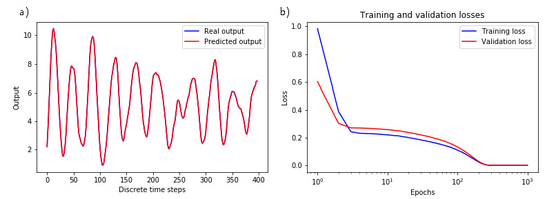
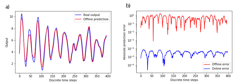
On lines 7 and 10 in the previous code list, we compute the prediction error and its percentage. Figure 1.a) shows the predicted and real outputs that are almost indistinguishable. The error is 0.0006%. Figure 1.b) shows the convergence of the training and validation losses. Furthermore, Fig.2.b) shows the error evolution during the prediction time.

Figure 1: a) The predicted and real output are almost indistinguishable. b) Training and validation losses.

When we performed the prediction, we used the real-system outputs. However, in many situations this might not be possible. Instead of using the real-system outputs to form the test data in the form of \eqref{dataPrediction}, we can use the past predicted output to compute future predictions. This is a so-called offline mode of the predictor. In the off-line mode we only use initial system measurements (real-outputs) during the first past horizon, and after that, we predict the system behavior using only past predictions. More precisely, the line 4 of the previous code, computes the following prediction at the time instant $i+p$:

$$\begin{align} \hat{y}_{i+p+1}=model.predict(\begin{bmatrix} u_{i+1} & u_{i+2} & \ldots & u_{i+p} & y_{i+1} & y_{i+2} & \ldots & y_{i+p} \end{bmatrix}) \label{predictionT1} \end{align}$$

Where the “hat” notation means that the output is predicted. However, instead of using the real-system outputs, we can use the past predicted outputs. In this case, the previous code line has the following form:

$$\begin{align} \hat{y}_{i+p+1}=model.predict(\begin{bmatrix} u_{i+1} & u_{i+2} & \ldots & u_{i+p} & \hat{y}_{i+1} & \hat{y}_{i+2} & \ldots & \hat{y}_{i+p} \end{bmatrix}) \label{predictionT2} \end{align}$$

As it is very-well known, this approach might suffer from instabilities in the sense that the predicted output after certain time will explode. The following code computed the predictions on the basis of the past predictions (offline mode). Notice that we used the system real outputs during the initial past horizon. This has to be done in order to initialize the predictor.

###############################################################################
#  do prediction on the basis of the past predicted outputs- this is an off-line mode
###############################################################################

# for the time instants from 0 to past-1, we use the on-line data 

predict_time=X_test.shape[0]-2*past

Y_predicted_offline=np.zeros(shape=(predict_time,1))
Y_past=network_prediction[0:past,:].T
X_predict_offline=np.zeros(shape=(1,2*past))

for i in range(0,predict_time):
    X_predict_offline[:,0:past]=X_test[i+2*past,0:past]
    X_predict_offline[:,past:2*past]=Y_past    
    y_predict_tmp= model.predict(X_predict_offline)
    Y_predicted_offline[i]=y_predict_tmp
    Y_past[:,0:past-1]=Y_past[:,1:]
    Y_past[:,-1]=y_predict_tmp

error_offline=Y_predicted_offline-Y_test[past:-past,:]
error_offline_percentage=LA.norm(error_offline,2)/LA.norm(Y_test,2)*100

#plot the offline prediction and the real output
plt.plot(Y_test[past:-past,:],'b',label='Real output')
plt.plot(Y_predicted_offline, 'r', label='Offline prediction')
plt.xlabel('Discrete time steps')
plt.ylabel('Output')
plt.legend()    
plt.savefig('prediction_offline.png')
#plt.show()

plt.figure()
#plot the absolute error (offline and online)
plt.plot(abs(error_offline),'r',label='Offline error')
plt.plot(abs(error),'b',label='Online error')
plt.xlabel('Discrete time steps')
plt.ylabel('Absolute prediction error')
plt.yscale('log')
plt.legend()   
plt.savefig('errors.png')
#plt.show()

The prediction performance in the offline model is shown in Fig.2.a). As expected the prediction performance is worse than in the online mode (when the predictor is performed using real system outputs in the past) shown in Fig.1.a). The offline error is 10.97 %. The errors for offline and online modes are shown in Fig.2.b).

Figure 2: a) The predicted and real output when the predicted output is computed using past predictions. b) Errors for offline prediction (when the prediction is performed using past predictions) and online prediction (when the prediction is performed using real outputs).